Learning-based 3D human kinematics estimation using behavioral constraints from activity classification

Participant & data collection for Exer

The IMUs (Bosch BNO0030, Bosch, Germany) were connected to the Beaglebone Black (Texas Instrument, USA) to measure 3D acceleration, 3D angular velocity, and 3D orientation (represented as 4D unit quaternions) data at 100 Hz. The quaternion values were obtained from the internal Kalman filter of the IMUs. Each IMU was mounted on a custom 3D printed case with four motion capture markers on each of the corners to determine the orientation of the IMU (Supplementary Fig. S1). IMU and OMC data were time-synchronized using a \(5{V}\) analog trigger signal. A \(5{V}\) signal was also used to obtain start and end times for each exercise, which were used for labeling the dataset prior to classification.

Data were collected on fifteen healthy participants (3 females; \(28.1\pm 5.6\) years) with two IMUs, one placed on their chest and one on their right wrist, to measure their 3D movement velocities and trajectories (Supplementary Fig. S1). Participants performed the following strength training exercises, each for 12 repetitions, in randomized order: Bench Press, Biceps Curl, Side Lateral Raise, Shoulder Press, Lat Pull Down, Squat, Barbell Lunge, Barbell Row, Triceps Curl, Dumbbell Fly, and Deadlift (Supplementary Fig. S2). The four sets were performed at four different self-selected movement speeds, normal, slow, fast, and variable. Six participants had one to three years of experience in strength training, another six had about one year or less of experience, and the remaining three had no prior strength training experience. While we provided instructions on performing the exercises before data collection, we did not verify whether the participants executed the strength training exercises with the correct form. We asked participants to place the sensors themselves and place them tightly to minimize movement during activities. Data were collected in accordance with Harvard Institutional Review Board (Protocol IRB-20-1847). We used data from 11 randomly selected participants for training and one participant for validation of the classification model. Data from the remaining three participants were used as the test dataset to evaluate the performance of the model.

Participant & data collection for Ind

Six participants (all males; \(30\pm 5.5\) years) wore three IMUs, one on their chest and another two on their right and left upper arms, to measure shoulder joint angles. Each participant performed 5 sets of overhead drilling, desk work (such as typing and note-taking), and treadmill walking (Supplementary Fig. S4). Each task was 3 minutes. We have “no action” as an additional label to indicate any activities performed transitioning among the three tasks. The time duration of “No action” between tasks was decided by each participant for each trial, ranging between 60 seconds to 90 seconds. We used Xsens MTI-3 IMUs collected at \(100{Hz}\). Each IMU was mounted on a custom 3D printed case with four motion capture markers on each of the corners (Supplementary Fig. S3). IMU and OMC data were time-synchronized using a \(5V\) analog trigger signal. This trigger also provided times for the start and end of a functional activity, which were used for classification. Data were collected in accordance with the Harvard Institutional Review Board (Protocol IRB19-1321). We performed LOOCV to assess the generalizability across participants. The training data included four participants, while the validation data included one person.

IMU and OMC coordinate frame definition

To ensure a fair comparison between IMU and OMC measurements, it is crucial to understand and align the coordinate frames of the two systems. As illustrated in Supplementary Fig. S10, the IMU sensor frame (SF) is defined by the physical placement of the sensing chip within the IMU, while its inertial frame (IF) is defined by the direction of gravity and the Earth’s magnetic North. Conversely, the body frame of OMC (BF) is defined by four markers rigidly mounted on the IMU case, and its lab frame (LF) is defined using an OMC L-frame calibration tool that was placed flat on the ground at the start of the data collection.

The relationship between the sensor and inertial frames of the IMU, and the body and LFs of OMC can be mathematically expressed as follows:

where \(q\) represents the unit quaternion of the coordinate frame in subscript, expressed in the coordinate frame in superscript. Specifically, \({q}_{{BF}}^{{LF}}\) and \({q}_{{SF}}^{{IF}}\) correspond to the OMC and IMU orientation measurements, respectively. The term \({q}_{{IF}}^{{LF}}\) and \({q}_{{BF}}^{{SF}}\) are the unknown misalignments between the IMU and OMC coordinate frames. These misalignments were determined using an optimization-based frame alignment method presented in our prior work²⁵.

For Ind, the 3D shoulder orientations are calculated using the following equation:

Where \({(q)}^{*}\) denotes the conjugate of quaternion \(q\), and \({q}_{{torso}}\) and \({q}_{{arm}}\) represent the unit quaternions of the torso and upper arm, respectively, as measured by either the IMU or OMC. This equation assumes that \({q}_{{torso}}\) and \({q}_{{arm}}\) are expressed in the same coordinate frame (IMU Inertial Frame in this case).

Detailed description of AIL-KE

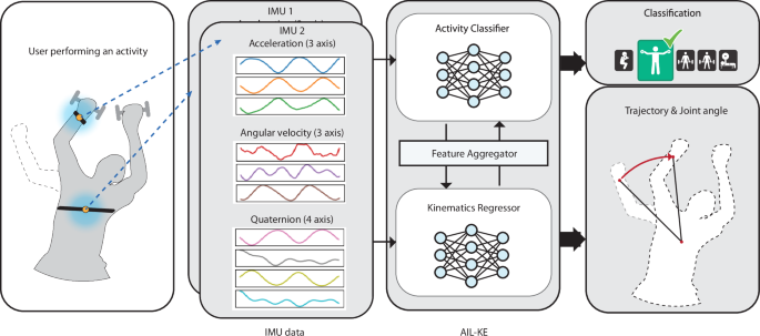
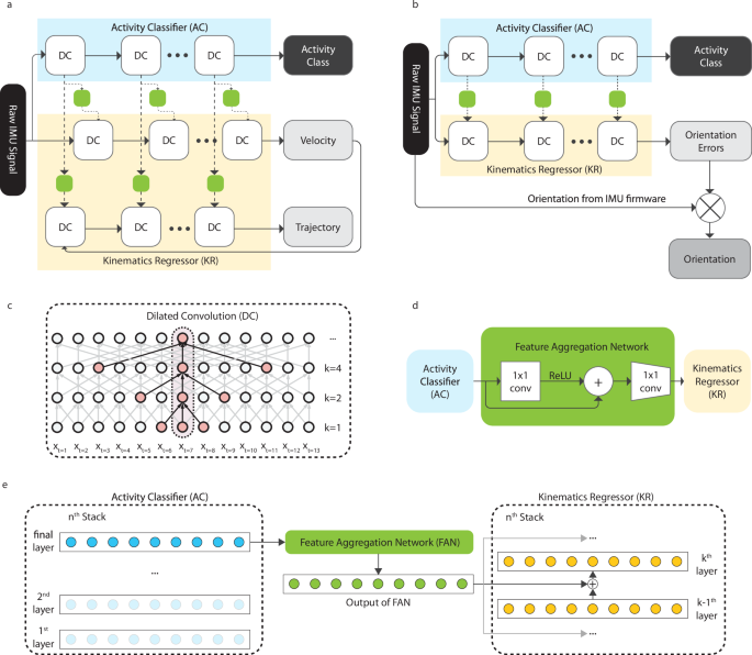
We present an end-to-end machine learning model incorporating human behavioral constraints for enhanced kinematics estimation using IMU sensors. In this study, we used two IMU sensors, but the number of IMU sensors for AIL-KE is not limited. We study two applications for AIL-KE: velocity and trajectory estimation (Fig. 4a) and 3-dimensional joint angle estimation (Fig. 4b). Although in this paper, we used separate models for trajectory and joint angle for specific purposes (i.e., Exer and Ind), these models can be merged to estimate all metrics in an end-to-end manner. The trajectory estimation model (Fig. 4a) used global accelerations, angular velocities, and quaternions from IMUs – one on the chest and the other on the wrist—as an input to predict 1) AC: exercise class \(\{{{{{\rm{c}}}}}_{1},…,{{{{\rm{c}}}}}_{{{{\rm{t}}}}}\}\) and 2) KR: velocity \({{{\rm{V}}}}=\{{{{{\rm{v}}}}}_{1},…,{{{{\rm{v}}}}}_{{{{\rm{t}}}}}\}\) and trajectory \(\Phi=\{{{{{\rm{\varphi }}}}}_{1},…,{{{{\rm{\varphi }}}}}_{{{{\rm{t}}}}}\}\) in each of the IMU global frames for every time frame t = 1, …, T, where T is the time length of each trial. The joint angle estimation model (Fig. 4b) used global accelerations, gyroscopes, and quaternions from the IMUs on the chest and each shoulder to predict activity class \(\{{{{{\rm{c}}}}}_{1},…,{{{{\rm{c}}}}}_{{{{\rm{t}}}}}\}\) for AC, and 2) quaternion angle errors \(\{{{{{\rm{e}}}}}_{1},…,{{{{\rm{e}}}}}_{{{{\rm{t}}}}}\}\) for KR at every time frame \(t=1,\,\ldots,{T}\). The output of KR is then multiplied by quaternions obtained through initial IMU calibration. AIL-KE is composed of stacked Dilated Convolutional Neural Networks, shown in Fig. 4a, b with DC (Fig. 4c)^50,51 and Feature Aggregation Network or FAN (Fig. 4d). Each Dilated Convolutional Neural Network, depicted in Fig. 4c, was composed of dilated 1-d convolutions⁵² with a dilation rate of \({2}^{0},{2}^{1},{2}^{2},\ldots,{2}^{d}\) and kernel size 3. This was followed by the Rectified Linear Unit (ReLU) activation function and a 1×1 convolution. The output of the 1×1 convolution is then summed with the input as a means of skip connection. The stacked dilated convolution structure allows the model to take temporal data with variable time lengths while the maximum dilation rate, i.e., \({2}^{d}\) must be smaller than the total time length of the one data sample, T.

a Overview schematic of how information from Activity Classifier (AC) is incorporated with Kinematics Regressor (KR) for velocity and trajectory estimation. b Overview schematic of how information from Activity Classifier (AC) is incorporated with Kinematics Regressor (KR) for joint angle estimation. c Detail view of Dilated Convolution layers (DC). The highlighted region in red shows how the features are operated in dilated convolution. d Detailed view of Feature Aggregation Network (FAN). 1×1 conv represents the one-by-one convolution layer, and ReLU represents the Rectified Linear Unit. e Detailed view of how features from AC are incorporated with KR through FAN.

FAN is a structure that provides activity classification information to KR (Fig. 4d). The last hidden layer (h_i) of each DCNN in AC was processed using FAN, which was summed with the output of each dilated convolutional neural network in KR. FAN was composed of point-wise convolution blocks and ReLU. Each h_i was fed into a one-by-one convolution layer, followed by ReLU. The output was summed with h_i as a residual structure, such that \({{{\rm{F}}}}({{{{\rm{h}}}}}_{{{{\rm{i}}}}})+{{{{\rm{h}}}}}_{{{{\rm{i}}}}}\), where \({{{\rm{F}}}}({{{{\rm{h}}}}}_{{{{\rm{i}}}}})\) is a 1×1 convolution. This was further processed by an additional 1×1 convolution layer to reduce depth size to fit into each DCNN in KR.

For every layer of DCNN, we used 1. \({{{{\mathcal{L}}}}}_{{AC}}\): the Categorical Crossentropy loss to minimize the classification error between ground truth and predicted for AC, and 2. \({{{{\mathcal{L}}}}}_{{KR}}\): the Mean Squared Error function to minimize the error between estimated and ground truth velocities and trajectories or joint angles for KR. The integrated loss equation is shown as follows:

Where \(s\) is \({s}^{{th}}\) stack given that \(s\in \{{{\mathrm{1,2}}},\ldots,S\}\), and N is the number of samples. V and \(\Phi\) are the ground truth velocity and trajectory that can be obtained from motion capture cameras, and \(\widehat{{{{\rm{V}}}}}\) and \(\widehat{\Phi }\) are the predicted velocity and trajectory based on IMU data.

For joint angle estimation, we used the following loss function for KR to minimize angular error, based on the quaternion inner product.

Where \({{{{\rm{q}}}}}_{{{{\rm{gt}}}}}\) is the ground truth quaternion obtained from the OMC and \({{{{\rm{q}}}}}_{{{{\rm{pred}}}}}\) is the quaternion obtained after normalizing the model-predicted orientation. This loss is reported to have numerical issues as there is a discontinuous gradient in the interval (−1, 1) at point 0, which results in extreme values at the points where \(\arccos (|{{{{\rm{q}}}}}_{{{{\rm{gt}}}}}\cdot {{{{\rm{q}}}}}_{{{{\rm{pred}}}}}|)\to 0\). Therefore, we used a gradient clipping approach, where the error derivative is clipped to a threshold during backpropagation through the deep learning network, and the clipped gradients are used to update the weights.

Model training strategy

We first trained AC for the first 500 epochs. Once AC was trained, we fixed the weights of AC and then trained KR for 1000 epochs. Then, AC and KR were trained together for another 500 epochs. We used 4 stacks of AC and KR. The hidden dimension was set to 64 for all layers, including DC and FAN. The maximum dilation rate for each stack was set to \({2}^{9}=512\). We used the Adam optimizer with a learning rate of \({10}^{-4}\) and weight decay of \({10}^{-7}\). These parameters were determined by grid searches.

Existing models for comparison

We compared the performance of the AIL-KE approach against the following models:

• DCNN: We used the same DCNN structure without FAN, i.e., we only used KR. The model architecture is shown in Supplementary Fig. S7.

• Long short-term memory (LSTM): LSTM is a Recurrent Neural Network architecture that has input, forget, and output gates in each of its nodes. The forget gate determines what information to retain or discard by applying a sigmoid function, which either multiplies by a factor of 1 or 0. These gates allow the network to handle long-range dependencies that arise from the vanishing and exploding gradient issues. LSTM structures are extensively utilized for time-series data processing^53,54,55, particularly for estimating position and angle based on IMU data. Hyperparameters of the LSTM, such as the number of layers and feature size, were found by grid searches. We used a 3-layer LSTM with a hidden feature size of 128, followed by two linear layers, each with a hidden feature size of 128.

• Transformer: The Transformer architecture has been widely used for training large language models⁵⁶. It is based on the scaled dot-product attention and self-attention mechanism, offering an alternative to traditional temporal models such as Recurrent Neural Networks. The hyperparameters, including the number of layers and feature size, were determined through grid searches. We used the encoder part of the Transformer, consisting of a two-layer Transformer with a hidden feature size of 128 and an attention head size of 8. Following the Transformer encoder, we added two fully connected layers with a hidden feature size of 256. The estimation results were tabulated in Supplementary Tables S1–S3.

• Xsens proprietary filter (Xsens): For angle estimation, we compared results from our model with the joint angle output from Xsens’ proprietary sensor fusion algorithm. Xsens is one of the world’s leading IMU companies and its proprietary algorithm is generally considered as the state-of-the-art. Joint angles were obtained by calculating the rotation matrices between chest and shoulder IMUs.

Orientation calculations

In the simulated industrial work experiment, the time-series motion magnitude was defined as the angular distance between the shoulder’s orientation at the initial time frame, \({q}_{{arm},0}^{{torso}}\), and its orientation at subsequent time frames, \({q}_{{arm},t}^{{torso}}\). Specifically, the motion magnitude at a specific time frame, \({\theta }_{t}\), is calculated using

where \({{\mathrm{Re}}}(q)\) denotes the real part of the quaternion \(q\).

Similarly, the time-series error profile for shoulder orientation was calculated as the angular distance between the estimated shoulder orientation and the ground truth. Specifically, the orientation error at a specific time frame, \({\psi }_{t}\), is calculated as

where \({q}_{{est},t}\) represents the shoulder orientation estimated by the machine learning model at time frame, \(t\), and \({q}_{{OMC},t}\) represents the ground truth orientation captured by the OMC system. This equation differs from Eq. 6 as it calculates angular distance at specific time frames, while Eq. 6 is a loss function for model training, leveraging numerical simplifications like the absolute operation for stability.

Statistical analysis on peak-to-peak errors

We calculated the peak-to-peak distances, i.e., the distance between the maximum and the minimum peaks, of the ground truth and AIL-KE, followed by calculating the RMSE between the positions of the ground truth and AIL-KE predictions. Then, the same operation was applied for DCNN and LSTM. We conducted the Mann–Whitney U test to determine statistical significance between the models, i.e., AIL-KE vs. DCNN, LSTM vs. DCNN, and AIL-KE vs. LSTM, using a significance level of 0.05.