Deep learning-based model for analyzing student engagement in activities

To offer accurate real-time student engagement analysis, it utilizes a multimodal educational dataset that includes digital activity logs, audio, video, and engagement labels. Video frames and digital logs are normalized using min–max scaling, while audio signals are subjected to median filtering. CNN-based feature extraction captures facial micro-expressions, action units, and behavioral signals, which are combined using the IAF2. The IC-BiSGRU-Net model classifies engagement into active, inactive, and disengaged states by merging BiLSTM, SGRU, and IC optimization. This enables precise and dependable monitoring, and it performs better and is more resilient than other models. Fig. 1 displays the overall process of analyzing student engagement in activities.

Overall process of analysing student engagement in activities.

Dataset

The multimodal educational dataset, which combines audio recordings, engagement labels, English learning performance, and privacy activity logs, is used to thoroughly examine student involvement. Speech-based behavioral signals are captured by audio data, whereas learning outcomes, involvement, and attentiveness are reflected in engagement and teaching statistics. Privacy logs provide contextual information and insights into system interactions, access patterns, and possible dangers. The dataset facilitates robust, multimodal engagement prediction for enhanced educational monitoring and interventions by combining these many modalities and supporting precise, real-time classification of active, inactive, and disengaged states. The datasets were splitted as Training Set (30%), Validation Set (15%) and Testing Set: (15%)

The three level engagement states are depending on multimodal indicators. Active engagement has an eye contact, high volume of micro-expressions, high volume of digital interactions, where at least two modalities have an increase in 70% features. Passive involvement demonstrates indifferent facial expressions, little verbal involvement, and medium log activity, which is equal to 30–69% activation. Depending on the level of activation ≤ 29% indicates disengaged students who lean their heads, yawn, speak little or no, and interact little or not at all. These quantitative threshold allow objective and multimodal categorizing of student engagement in real-time learning situations.

Source:

Data pre-processing steps

Pre-processing of the data included median filtering of audio signals to minimize noise and min–max normalization of video and digital activity log characteristics to guarantee balanced scaling. These actions increased the accuracy of engagement detection, maintained key signals, and improved feature comparability. as well as eliminating superfluous variants, cutting down on repetition, and guaranteeing resilience across diverse datasets. To provide consistent, scalable, and adaptable engagement monitoring solutions in both conventional classroom settings and quickly changing online learning environments, preprocessing also made it possible to integrate multimodal inputs efficiently, streamline downstream model training, and improve the generalizability of predictive outcomes.

Min-max normalization

Min-max normalization is used to normalize features from digital activity logs and video frames, resulting in balanced feature contributions for model training that offer a precise, reliable, and real-time analysis of student engagement. Parameters like pixel intensities, facial action units, click counts, and interaction durations are transformed linearly to produce a common range. Equation (1) expresses the transformation:

Here, \(\:{u}^{{\prime\:}}\) is the normalized value of the feature, \(\:u\) is the original feature value, \(\:{max}_{B}-{min}_{B}\) is the minimum and maximum values of the feature \(\:B\), \(\:ne{w}_{{min}_{B}},ne{w}_{{max}_{B}}\)​​ is the new desired range (typically 0–1), and \(\:{u}^{{\prime\:}}\) is the normalized feature value. This normalization procedure ensures fair scaling across visual and interaction-based components, which enhances model training, feature comparability, and engagement prediction in student engagement analysis.

Pre-processed digital logs using Min-Max normalization.

By employing min–max normalization (0–1 range) to normalize the digital activity data from logs and video frames, balanced contributions, better comparability across features, and increased accuracy and reliability in forecasting student involvement were all achieved in Fig. 2. It highlighting consistent scaling, reduced bias, and enhanced interpretability for subsequent analytical modeling processes. Technique improves real-time engagement analysis, classification reliability, and accuracy by guaranteeing that visual signals contribute fairly throughout model training, supporting robust feature integration, minimizing distortions, and enabling scalable deployment of engagement detection frameworks across diverse educational platforms and learning contexts.

Median filtering

The median filter was used as a noise reduction method to enhance the quality of multimodal data for student engagement evaluation. The median filter, the most well-known order-statistics filter, substitutes the median of the values in a sample’s neighborhood for the value of a sample in an audio signal. When calculating the median, the original value is taken into account and is represented as follows in Eq. (2):

Where, \(\:\stackrel{\sim}{e\:}\left(W,Z\right)\:\)is the original value of the sample (audio amplitude) at location \(\:W,Z\:\), median​ is the new value after applying the median filter. \(\:h\:(t,s)\) is the original audio values around. \(\:{S}_{wz}\) is the Neighborhood of samples. \(\:\left(t,s\right)\in\:\) is the median value of all samples in that neighborhood, which replaces the original value. This technique supports accurate engagement detection by offering strong noise reduction for random environmental disturbances in audio while maintaining crucial information like speech cues and temporal patterns.

Effect of median filtering on audio signals.

To reduce noise while maintaining speech patterns and temporal clues for precise student engagement analysis, the original signal with noise spikes (left) is smoothed (right) in Fig. 3, which demonstrates median filtering on audio. This shows how to apply median filtering to audio to efficiently preserve important acoustic characteristics, lessen distortion, and maintain minor prosodic fluctuations. By supplying cleaner, more trustworthy input data, this preprocessing phase improves the performance of the downstream model, increasing classification stability and guaranteeing precise interpretation of engagement-related auditory behaviors across a variety of online and classroom learning situations.

Feature extraction using convolutional neural network (CNN)

The CNN is a structural neural network with several layers, including layers for classification, pooling, and convolution. To capture delicate emotional and attentional indicators, CNNs are used to extract action units and face micro-expressions from classroom video recordings. These visual elements are paired with digital activity logs, which record interaction patterns including click counts and activity durations, and audio interactions, which offer speech-based behavioral indications. The CNN-based feature extraction procedure supports the model in categorizing engagement into active, passive, and disengaged states by combining various multimodal sources and enabling thorough, real-time analysis of student involvement. Following processing, the video data goes through convolutional and pooling layers, which remove duplicate information and extract action units and face micro expressions to identify significant patterns. These characteristics are progressively combined. The collected visual elements are merged with normalized digital activity logs and audio exchanges to provide sequential behavioral cues. Ultimately, a completely linked layer receives the integrated multimodal information and uses it to categorize each instance into active, passive, or disengaged states in real time, as well as to generate forecasts for student participation.

Digital logs CNN feature map visualization.

CNN feature maps that were taken from digital activity records are shown in the scatter plot in Fig. 4. Different interaction patterns, including click counts and durations, are captured by each filter. Accurate, real-time engagement categorization is improved by these normalized activations, which improve multimodal fusion with audio and video signals. allowing for the thorough modeling of behavioral dynamics. The Predictive generalizability is improved, feature imbalance is decreased, and pattern recognition is strengthened by the integration of many modalities. Additionally, by enabling the system to dynamically adjust to different interaction situations, these representations enhance scalability across educational environments and provide robust detection of subtle behavioral inputs.

Image CNN feature map visualization.

CNN feature maps from classroom video frames are displayed in the scatter plot, with each filter capturing unique pixel-level patterns in Fig. 5. When combined with digital and audio records, these extracted features, which stand for face micro-expressions and action units, enable precise real-time categorization of student engagement. The personalized learning and adaptive therapies are supported by the multimodal integration, which improves the detection of subtle behavioral and emotional clues. By ensuring uniformity across a range of lighting situations, camera angles, and classroom environments, normalized feature representations increase resilience. Additionally, scalable analysis is made possible by these coupled activations, enabling ongoing observation of engagement trends for both individual students and larger class sizes.

Iterative attentional feature fusion (IAF2)

A strong classification of student involvement into active, inactive, and disengaged stages requires the inclusion of high-quality multimodal features. Engagement prediction performance is strongly impacted by the quality of feature integration. Fully context-aware fusion, in contrast to partially context-aware methods, faces the difficulty of successfully integrating disparate input elements (video, audio, and digital activity logs) at the outset. It makes sense to use an additional attention technique to improve integration, as the task remains a feature fusion challenge.

The model of iterative attentional feature fusion (IAF2).

This two-step process is called Iterative Attentional Feature Fusion (IAF2) and is illustrated in Fig. 6. The original multimodal feature integration can be rephrased as follows in Eq. (3):

Here, \(\:W\) is the Features from video facial micro-expressions and action units extracted. \(\:Z\) is the Features from audio and digital activity logs. \(\:N\:\)is the Attention weights that determine how important each modality is when combining \(\:W\:and\:Z\). \(\:\otimes\) is the Element-wise multiplication to apply the attention weights to each modality. \(\:W \uplus Z\) is the final combined feature representation after iterative attentional fusion. In the IAF2 process, Multi-Scale Cross-Attention Module (MS-CAM) helps the network iteratively refine the fusion of multimodal features, improving engagement classification performance.

Proposed model

To improve student engagement prediction, the suggested IC-BiSGRU-Net framework uses a hybrid optimization approach that combines Improved Chimp Optimization (IC), Scalable Gated Recurrent Unit (SGRU), and Bi-directional LSTM (BiLSTM) with dynamic weighting. BiLSTM ensures contextual knowledge from past and future states by capturing both forward and backward temporal dependencies in sequential multimodal inputs, such as action units, audio, digital interaction logs, and facial micro-expressions. By minimizing learnable parameters for real-time analysis and preventing gradient vanishing and explosion, SGRU effectively models spatiotemporal patterns while maintaining early behavioral signals. While dynamic weighting gives candidate solutions proportionate weight depending on their contribution to the optimal solution, IC optimization uses a somersault technique to adaptively fine-tune network parameters, allowing escape from local optima. The hybrid IC-BiSGRU-Net MODEL ensures faster convergence, enhanced robustness, and accurate classification of student engagement into active, passive, and disengaged stages. A reliable and efficient real-time engagement prediction system that performs well in a range of educational contexts is produced by this approach. Algorithm 1 extracts and fuses multimodal features, applies attention mechanisms, and utilizes a bidirectional GRU with improved initialization to efficiently classify student engagement as active, passive, or disengaged.

Hybrid IC-BiSGRU-Net model.

Scalable gated recurrent unit (SGRU)

To accurately model temporal correlations in multimodal student engagement information. Typical recurrent models cannot capture the short- and long-term correlations seen in engagement signals such as interaction logs and facial expressions due to vanishing gradients and early cue forgetting. An Enhanced Gated Recurrent Unit (EGRU) to get around this. Its attention component maintains early behavioral cues, and its gating mechanism controls the flow of information, allowing for reliable real-time categorization of active, passive, and disengaged states, as shown in Fig. 7.

The improved gated recurrent unit takes as inputs \(\:{G}_{s-1}\:\), \(\:{W}_{mgc}\), and \(\:{\mathcal{W}}_{S}^{{\prime\:}}\:\:\). At moment \(\:s-1\:\), \(\:{G}_{s-1}\:\)is the hidden state that contains the engagement feature information. The input data following dimension elevation \(\:{\mathcal{W}}_{S}^{{\prime\:}}\), preserves the original temporal engagement patterns, whereas \(\:\:{W}_{mgc}\) reflects spatial information such facial action units and micro-expressions obtained from multimodal inputs. By employing \(\:\:{W}_{mgc}\) to calculate the reset gate \(\:q\)in the improved gated recurrent unit, pertinent engagement data from the prior state can be retained. Attention scores compute the update gate \(\:\:y\:\) by combining \(\:\:{W}_{mgc}\) and \(\:{G}_{s-1}\) to create \(\:{W}_{st}\). To ensure precise tracking of active, passive, and disengaged behaviors across time, the update gate controls the amount that previous engagement data affects the present state.

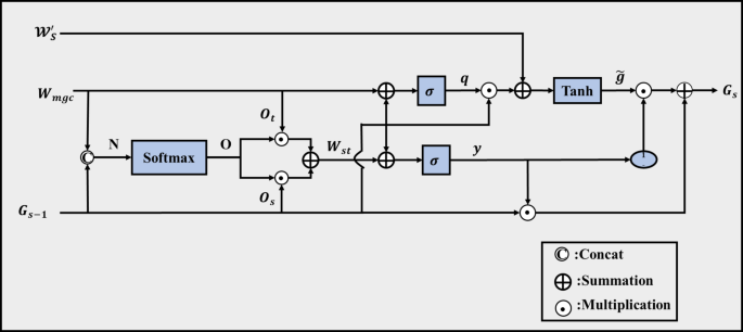
The scalable gate recurrent unit structure.

The following is the computing procedure used to determine the attention scores needed to combine \(\:{W}_{mgc}\:\) and \(\:{G}_{s-1}\)into \(\:{W}_{st}\), which includes rich behavioral and temporal engagement features: Formula (9) illustrates that \(\:N\) is obtained by splicing \(\:{W}_{mgc}\:\)is multimodal spatial features taken from facial expressions, micro-expressions, and action units with \(\:{G}_{s-1}\) is prior hidden state conveying past engagement context in Eq. (4):

The softmax function is used to calculate the attention scores, which are given as follows in Eq. (5):

Where, \(\:O\:\)is the attention scores showing the importance of each feature. \(\:N\) is the input values from combined features. \(\:softmax\:\)is an activation function. The tensor splitting procedure in this case is \(\:split\left(O\right)\), where \(\:{O}_{t}\) is equivalent to \(\:{W}_{mgc}\:\)and \(\:{O}_{s}\)is is equivalent to \(\:{G}_{s-1}\). Ultimately, the combination of temporal states and multimodal properties is as follows in Eq. (6):

Where \(\:{W}_{st}\) stands for the combined feature vector that incorporates previous contextual states as well as current engagement signals. By limiting the omission of pertinent signals during gate updates, the use of \(\:{W}_{st}\) in the update gate guarantees the preservation of important engagement-related data. The following is an expression for the procedure of updating the hidden state with \(\:{\mathcal{W}}_{S}^{{\prime\:}}\:\:\)and determining the gate units using \(\:{W}_{mgc}\) and \(\:{W}_{st}\):

Where, Eq. (7) \(\:q\) is the reset gate controlling retention of prior engagement information. \(\:y\) is the update gate determining the influence of past states on the current state. \(\:\stackrel{\sim}{g}\) is the candidate hidden unit representing potential new engagement features. \(\:{G}_{s}\) is the hidden state at the current moment, containing updated temporal and multimodal engagement information. \(\:\sigma\:\) is the sigmoid activation function. \(\:\text{T}\text{a}\text{n}\text{h}\:\)(Hyperbolic tangent) is an activation function. \(\:{X}_{q}\)is input features for the reset gate (video, audio, digital logs, or combined features). \(\:{W}_{mgc}\:\)is the learnable weight matrix for the reset gate. \(\:{V}_{q}\)is the learnable weight matrix for the previous hidden state contribution. \(\:{G}_{s-1}\)is the previous hidden state containing past engagement features. \(\:{X}_{y}\) is the input feature for the update gate. \(\:{W}_{st}\)is the learnable weight matrix for the update gate. \(\:{V}_{y}\) is the learnable weight matrix for the previous hidden state contribution. \(\:{X}_{g}\) is the input features for the candidate unit. \(\:{\mathcal{W}}_{S}^{{\prime\:}}\) is the learnable weight matrix for the applicant unit. \(\:{V}_{g}\) is the weight matrix applied to the gated previous hidden state\(\:\:1-y\) is the proportion of the candidate hidden unit contributing to the current hidden state. The improved gated recurrent unit records spatiotemporal characteristics from multimodal inputs, such as interaction logs, action units, and face microexpressions. Early engagement cues are preserved, gradient vanishing or explosion is mitigated, and the loss of correlation information during temporal propagation is minimized due to its gate computation technique. Furthermore, by removing bias factors from the update formula, the SGRU model’s efficiency and robustness for real-time student engagement analysis are improved by reducing the number of learnable parameters.

Bi-directional long short-term memory network (Bi-LSTM)

The BiLSTM was used to record sequential student data to capture both past and future engagement factors. In Fig. 8, to improve the temporal modeling of student involvement, BiLSTM integrates information from prior and subsequent times by processing sequential data in both forward and reverse directions, in contrast to regular LSTM, which considers only past information.

Structure of the BiLSTM module.

Both forward \(\:\overrightarrow{{g}_{s}}\:\)and backward \(\:\overleftarrow{{g}_{s}}\) hidden layer activations are included in the BiLSTM hidden layer output. The expression for BiLSTM is as follows in Eq. (8) to (10):

Where, \(\:{w}_{s}\:\)is the input feature at time \(\:s\), including multimodal engagement cues (facial expressions, micro-expressions, action units, and interaction logs). \(\:\overrightarrow{{g}_{s}}\) and \(\:\overleftarrow{{g}_{s}}\) are the forward and backward hidden states at time \(\:s\), capturing past and future context, respectively. \(\:{G}_{s}\:\)is the combined hidden layer output used for engagement prediction. \(\:\sigma\:\) is the initiation function. \(\:{X}_{w\overrightarrow{g}}{w}_{s}\) is the weight matrix connecting input features.\(\:{X}_{\overrightarrow{g}\:\overrightarrow{g}}\overrightarrow{{g}_{s-1}}\) is the forward hidden state. \(\:{a}_{\overrightarrow{g}}\) is the Bias vector for the forward hidden state. \(\:{X}_{w\:\overleftarrow{g}}{w}_{s}\) is the weight matrix connecting input features. \(\:{X}_{\overleftarrow{g}\:\overleftarrow{g}}\overleftarrow{{g}_{s-1}}\) is the backward hidden state. \(\:{a}_{\overleftarrow{g}}\) is the bias vector for the backward hidden state.\(\:{X}_{w\overrightarrow{g}}\overrightarrow{g}\) is the contribution of the forward hidden state \(\:\overrightarrow{g}\:\) after applying the weight matrix. \(\:{X}_{\overleftarrow{g}\:\overleftarrow{g}}\overleftarrow{{g}_{s-1}}\) is the contribution of the backward hidden state \(\:\overleftarrow{g}\:\)after applying the weight matrix. \(\:{a}_{z}\) is the Bias vector, adjusting the combined hidden output \(\:{G}_{s}\)​ for final activation. The BiLSTM model enhances temporal modeling by taking into account both past and future data, making it possible to forecast active, passive, and disengaged student engagement states in real-time educational environments with more accuracy and resilience.

Intelligent chimp optimization (ICO)

The Intelligent Chimp Optimization (IC) method was used to adaptively fine-tune network parameters to increase the accuracy and convergence for student engagement analysis. The first Chimp Optimization Algorithm could eventually converge to a local optimum.

Somersault foraging strategy

ùe ability to perform somersault to avoid local optima and move closer to the global optimum, an approach inspired by the leaping behavior of monkeys in the Monkey Algorithm (MA). Once a local optimal solution has been found, a chimp uses a distance coefficient and a particular support point to execute a somersault, which causes the network parameters to leap out of the local optimal zone. The fulcrum in this optimization method stands for the local optimum, whereas the current location of the network parameters indicates the chimp’s position. The flowchart of ICO as shown in Fig. 9.

Flowchart of intelligent chimp optimization (ICO).

To improve engagement prediction performance and allow for a more thorough investigation of the parameter space, updated parameter locations are calculated between the present position and the position symmetric to the center. The following Eq. (11) illustrates the mathematical model for adaptively fine-tuning the parameters using \(\:{w}_{j}^{c}\left(s+1\right),\:\)the somersault strategy:

Where, \(\:{w}_{j}^{c}\left(s\right)\) is the current position of the \(\:{j}^{th}\) chimp in dimension \(\:c\) at iteration \(\:s\), representing the current network parameter value. \(\:{w}_{j}^{c}\left(s+1\right)\) is the efficient location of the \(\:{j}^{th}\) chimp in dimension \(\:c\:\)at iteration \(\:s+1\), representing the new network parameter value after the somersault. \(\:{w}_{j}^{c}\left(s\right)\:\)represents the current value of the network parameter. \(\:T\) is the somersault factor, determines the distance and direction to jump from the local optimum; \(\:{w}_{best}^{c}\left(s\right)\) is the prey position, representing the local optimum (fulcrum) in the parameter space. \(\:M\) is the Number of chimps, representing the population size of candidate solutions. \(\:c\) is the Dimension of the search space, corresponding to the number of network parameters being optimized. \(\:{q}_{1}\)​,\(\:{q}_{2}\) are the random numbers in [0,1] to introduce stochasticity in exploration.

Dynamic weighting factor

In the Improved Chimp Optimization (IC) method, a dynamic weighting component was added to enhance the adaptive fine-tuning of network parameters. The first position update ignores the various contributions made by individual chimps and treats equally, as the population gets closer to the ideal solution. Based on the step length Euclidean distance, the suggested dynamic weight assigns a relative priority to each chimp, representing its impact on determining the global optimum.

The optimization capability can be improved by adding this dynamic weighting element to the position update equations, which speeds up convergence and raises the forecast accuracy of student participation. The method ensure that chimps that make a larger contribution to the best solution have a proportionately greater influence on changing the network parameters, whereas chimps that are less successful make a smaller contribution. The dynamic weight is generated from the coefficient vectors \(\:B\) and \(\:D\:\)in ChOA, as opposed to the proportionate weight based on step length Euclidean distance, it generates weights from the predator’s position. Throughout the optimization process, the weight factor changes non-linearly due to the dynamic and unpredictable nature of these vectors, which directly regulate the search range for the ideal network parameters. \(\:{B}_{1},{B}_{2},{B}_{3},{B}_{4}\:\:\)are different from \(\:{D}_{1},{D}_{2},{D}_{3}\:\:{D}_{4}\:\:\:\)in the basic ChOA. \(\:\:{B}_{1},{B}_{2},{B}_{3}\:\:{B}_{4}\:\)in Eq. (12) and \(\:{D}_{1},{D}_{2},{D}_{3},{D}_{4}\:\)in Eq. (13) are used to guarantee relevance in weight updates, where \(\:e\) is the linearly decreasing factor governing exploration and exploitation and \(\:{q}_{1}\) and \(\:{q}_{2}\) are random values that fall inside [0,1].

The intended dynamic weighting factors for the position vectors are calculated as follows to enhance the IC network parameters in Equations (14) to (17):

Where, \(\:{\omega\:}_{1}\), \(\:{\omega\:}_{2}\), \(\:{\omega\:}_{3}\), \(\:{\omega\:}_{4}\) are the Dynamic weighting factors for the four candidate positions. \(\:{B}_{1}\), \(\:{B}_{2}\), \(\:{B}_{3}\), \(\:{B}_{4}\) are the Coefficient vectors controlling exploration in the IC optimization \(\:{D}_{1}\), \(\:{D}_{2}\), \(\:{D}_{3}\), \(\:{D}_{4}\) are the Coefficient vectors controlling the predator search range in IC optimization. The updated position vector is calculated as follows in Eq. (18):

Where, \(\:w\left(s+1\right)\:\)is the updated network parameter vector after applying dynamic weights. \(\:{w}_{1}\), \(\:{w}_{2}\), \(\:{w}_{3}\), and \(\:{w}_{4}\) are the candidate network parameter vectors generated in the current IC iteration. \(\:{\omega\:}_{1}\), \(\:{\omega\:}_{2}\), \(\:{\omega\:}_{3}\), and \(\:{\omega\:}_{4}\) are the dynamic weighting factors applied to each candidate vector. The IC optimization method improves convergence, accuracy, and search space exploration for efficient student engagement prediction by adaptively adjusting network parameters using tumbling techniques and dynamic weighting.

The hybrid IC-BiSGRU-Net MODEL guarantees improved robustness, quicker convergence, and precise differentiation of student involvement into active, passive, and disengaged phases. This method creates a dependable and effective real-time engagement prediction system that performed well in a variety of educational contexts, while facilitating the smooth integration of multimodal inputs, reducing processing cost, and supporting adaptive interventions for ongoing, scalable monitoring of a variety of learner behaviors.

Table 2 summarizes the key hyperparameters applied during model training, including learning rate, batch size, epochs, network units, and dropout, which collectively support optimized learning performance, stability, and generalization of the IC-BiSGRU-Net model.